Efficiently finding candidate partitions for point queries

Efficient Execution of Point Queries in Large Tables

Summary

In this blog post, we present an efficient way to accelerate point queries on large Parquet-based tables consisting of millions of files. By utilizing aligned arrays of Cuckoo Filters, we aim to identify files that likely have the data you’re looking for, using only two read operations, while keeping all your index data on disk.

Depending on the latency of the underlying storage layer, we are able to identify relevant data files in milliseconds, enabling a query engine to only consider a small fraction of the original data, speeding up needle-in-a-haystack queries by orders of magnitudes.

We validate our approach with an experimental implementation, and benchmarks on artificial datasets of various sizes and configurations.

Motivation

Table formats like Delta Lake or Apache Iceberg provide efficient storage for large amounts of data leveraging columnar file formats like Parquet, and are optimized for analytical queries and batch-processing of data.

Due to efficient compression techniques, storing data in a columnar format can also be attractive for data that does not fit the “analytical processing” paradigm, by reducing storage cost or making it possible to store data that would otherwise be infeasible. This includes network telemetry, structured service logs, or similar event-centric data that comes in large quantities.

Unfortunately, this type of data is often queried in ways that would be better served by a database, backed by a secondary index: How do you find all the logs related to a specific request ID, or all hosts in your network that established a connection to a newly identified botnet?

In a sea of Parquet files, without additional information, the only option is a full table scan. There’s a variety of mitigations and workarounds, like data partitioning, or leveraging column statistics at the file level, but this typically involves optimizing the data layout for a few specific types of queries from the get-go, and is not always practical if data is used for more than one purpose or queried on multiple columns. Can we do better?

Approximate Membership Query Filters

Bloom filters and related datastructures are a great fit for this type of problem: a very compact representation of a set of values (e.g., all values of one column in a Parquet file or other chunk of a table), that allows for approximately checking a value to either maybe exist in a set or definitely not exist in the set.

By creating such a filter for every Parquet file, it is possible to trim down the number of files to read by first consulting all filters. Databricks provides this feature by maintaining a separate index file per Parquet file, and can skip reading irrelevant files all together. A similar approach is specified as part of the Parquet format, where bloom index pages are defined as part of the row group metadata of each Parquet file. However, both approaches are tied to the Parquet format. Since they maintain the index data in a one-to-one relationship with the associated Parquet file, they require making one read request for each candidate file to check the filter, leading to excessive I/O if the initial set of candidate files is large.

We can work around the I/O burden by keeping the Bloom filters in memory. The downside here is that the memory requirements for your index grow with the amount of data you want to store; a single Bloom filter for 1 million elements can grow over 1.7MB even for a modest false positive rate of 0.1%. With one million files, that’s almost 2TB of index data to keep in memory, which also has to be pre-loaded before a query can even start executing. Even if there is sufficient memory available, evaluating a million independent Bloom filters translates to millions of single-bit reads on more or less random memory locations, which is not nearly as fast as you would come to expect from “in-memory” operations.

A Better Approach

Ideally, we want to have the performance of in-memory bloom filters, but we don’t want to keep the index data in memory; we need a data structure that allows us to perform approximate membership queries for a single value on many sets simultaneously, while keeping the index data on disk and avoiding a separate read operation for each individual set.

The motivational examples start from a set of Parquet files. When the index is stored independently from the indexed data, it is not necessary to limit ourselves to indexing a single column of a Parquet file, but any chunk or subset of a table that can be sensibly processed separately. This could be other file types (avro, orc, csv, …), or an individual row group in a Parquet file. We will from now on refer to identifying candidate partitions.

Cuckoo Filters: An Alternative to Bloom Filters

Cuckoo Filters (see paper) provide a useful improvement over Bloom filters for our use case, as they only require two read operations for a single-value lookup - Bloom filters require a number of lookups that depends on the desired false-positive rate (you can try out a Bloom filter calculator over here). There’s also an introduction to Cuckoo Filters with some animations on brilliant.org.

We will use a small variation on the original Cuckoo Filter implementation that allows us to grow the number of slots per bucket, to encode sets of different sizes using the same number of buckets. This is necessary in case the Parquet files to index are varying in size or number of distinct values in the indexed column.

A single Cuckoo Filter with two buckets for a value x

In the example above, we sketched a Cuckoo Filter with six buckets and two slots, providing a capacity for 12 entries. Each entry stores the fingerprint of a single value, and each value is mapped to both a fingerprint and two buckets.

A lookup for a value x computes the two candidate buckets and checks all slots of these two buckets for its fingerprint. A collision (false positive) occurs when another value has the same fingerprint in one of the two buckets. The false positive rate fp of the Cuckoo Filter is thus determined by the bucket size b and the size of the fingerprint in bits, fb:

\[\text{fp} = \frac{2 b}{2^{fb}}\]

In other words, for a fixed number of distinct values in a set, we can reduce the false positive rate by increasing the size of the fingerprint, or by increasing the number of buckets to bring the bucket size b down. On the other hand, a small bucket size b reduces the expected table occupancy. According to the paper, bucket sizes of b = 1, 2, 4 and 8 lead to expected occupancies of 50%, 84%, 95%, and 98 respectively.

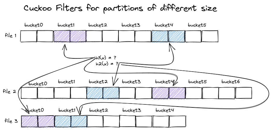Multiple Cuckoo Filters of different size access different buckets for the same value

Creating an optimal Cuckoo Filter for several sets of values of different sizes leads to a different choice in the number of buckets in each filter, as depicted above. The hash function that selects candidate buckets depends on the number of buckets, resulting in different selected buckets for the different filters, even when looking up the same value x.

Aligning Cuckoo Filters

The previous image shows how evaluating a number of Cuckoo Filters for partitions of different sizes leads to all the problems we initially described for the Bloom filter approach: we have to search for a given fingerprint in a bunch of mostly random memory locations - trying this with index data stored on disk will not perform well, and we’ll have to compute hash functions $h_1$ and $h_2$ for every filter individually.

To overcome the irregularity of the data layout, we can try to keep the number of buckets per filter constant, which leads to a much more regular structure:

Cuckoo Filters with aligned bucket sizes

When all individual filters have the same number of buckets, a few things change:

• $h_1(x)$ and $h_2(x)$ point to the same two buckets for all filters
• to make room for the additional elements in the second filter, we increased its bucket size
• we give up on some optimality in occupancy:
  • filter 2 has 18 instead of 12 entries overall
  • filter 3 has 12 instead of 10 entries overall
• false positive rate for filter 2 has increased alongside bucket size

Evaluating the set of filters now only requires a single computation of $h_1(x)$ and $h_2(x)$ each, and the memory accesses for each selected bucket are evenly spaced.

However, the index still only evaluates a few entries here and there, either reading unnecessary data or making lots of independent micro-sized read requests. To make everything fall into its proper place, we need one last trick.

Bucket-Major Data Layout

To reduce the number of read operations and utilize sequential reads, we change the layout of our data: instead of storing all index data for the first file, followed by all index data for the second file, we store all index data for the first bucket, followed by all index data for the second bucket, and so on. Now, all data for the two buckets that are needed to identify candidate partitions is in only two places, each containing a long stream of fingerprints representing the data of a single bucket, but for all files or partitions at once:

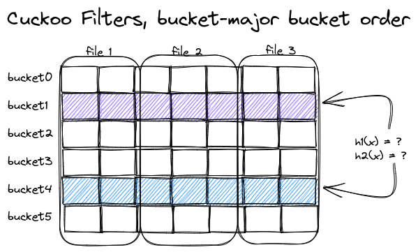Beautifully aligned access pattern and memory layout

Conclusion

We made some progress in this section: we found a representation of the index data that avoids costly random reads, but does not require the index data to reside in memory. How does it perform? We’ll look at some benchmarks in the next section.

Benchmarking

We implemented our approach as a proof of concept, available on github. It currently only supports data stored on a file system, and there’s no write-ahead log or recovery strategy. The index only stores 64-bit unsigned integer values - the assumption is that columns of other data types are hashed to represent them as u64. Since the index is only used to identify candidate files or data partitions and may already contain false positives anyway, a hash collision at the level of the actual data poses no fundamental problem.

We store two principal types of data:

1. Bucket data, which is a sequence of 16-bit fingerprints, maintained in a separate file per bucket.
2. Partition metadata, which contains a partition identifier, a removed flag and, crucially, the bucket size of that partition. The latter is important because you need to be able to restore which partition a matching fingerprint actually belongs to - the information “we have a matching fingerprint in position 3192” is not sufficient.

While the index data remains on disk, the partition metadata resides in-memory, and clocks in at 25 bytes per partition for the benchmark implementation. The actual size depends on how you want your partition to be identified. Storing the path or URI to a Parquet file requires more space than a storage layout where a UUID is sufficient to identify a partition.

We only benchmark the index itself - there’s no actual Parquet files with real data, and artificial data is crafted in a way that allows recreating the entire large dataset from a small set of parameters: the number of partitions p, the number of elements per partition e, the number of buckets b. A single partition used in the benchmarks just describes a consecutive range of values:

#[derive(Debug, Clone, PartialEq, serde::Serialize, serde::Deserialize)]
pub struct BenchmarkPartition {
    pub start: u64,
    pub length: u64,
}

This allows us to verify correctness even for large datasets, because we know which values belong to which partitions, and computing a false positive rate is equally simple. Since both the fingerprint and the bucket location of the stored values are derived via hash functions, the fact that a partition contains a consecutive range of values should have no meaningful impact on the benchmark runs. Not storing actual data allows us to simulate datasets with up to 100 billion entries, consuming only 250GB from our limited benchmark hardware.

We look at the query performance, false positive rate and occupancy of datasets of varying number of partitions, number of buckets, and size of each partition. Finally, to test the ability to serve multiple read requests, we measure query performance in a multi-threaded fashion.

Benchmarks have been performed on a Thinkpad P14s with an AMD Ryzen 7 Pro 5850U CPU and 48GB of memory. All tests used the local NVMe SSD.

Overall Performance

To get us started, we’re simulating a dataset with 100k distinct values per partition. We configure the index to have 38000 buckets, and expect that each partition has a resulting bucket size of approximately 3. This is not always the case: it seems that for about 10% of the partitions, partition’s bucket size grows to occupy 4 slots. The overall occupancy was about 0.8, so we’re wasting quite a bit of space.

Here’s the query latency for a single-threaded run with varying number of partitions:

Index size	#Partitions	Bucket size	#Buckets	Latency ms
$1 \times 10^{10}$	100000	327060	38000	0.527
$2 \times 10^{10}$	200000	654235	38000	2.307
$3 \times 10^{10}$	300000	981886	38000	4.346
$4 \times 10^{10}$	400000	1308534	38000	6.304
$5 \times 10^{10}$	500000	1635382	38000	9.267
$6 \times 10^{10}$	600000	1963086	38000	9.793
$7 \times 10^{10}$	700000	2289914	38000	10.371
$8 \times 10^{10}$	800000	2616379	38000	13.153
$9 \times 10^{10}$	900000	2944014	38000	15.010
$10 \times 10^{10}$	1000000	3271554	38000	17.758

For one million partitions, we can retrieve candidate partitions results in less than 20 ms. This is a great result, given that the index contains 100 billion entries, but keep in mind that the partitions where all equally sized and the bucket size was configured to perfectly match the partition size, leading to buckets that are as small as possible. We’ll look into the effect of varying the number of buckets in the next section.

The first experimient with 100k partitions is 4x as fast as the next one, despite only a factor of 2x in the index size: I’m attributing this to the file system cache, which is able to keep the entire index cached for the first run, but doesn’t quite fit the larger index sizes - and its effect is successively getting smaller the larger the data set.

Let’s look into how varying the number of buckets affects query performance.

Number of Buckets

A query execution for finding all partitions containing a specific value x has to search for the fingerprint in exactly two buckets, and all buckets are equally long. The bucket size depends on:

1. The number of buckets: if fingerprints are distributed over more buckets, each bucket contains less fingerprints.
2. The number of elements in each partition: more data leads to longer buckets
3. The number of partitions: each partition just appends its data to all buckets

The work that needs to be done depends on the number of fingerprints in each bucket, and we expect a mostly linear relation between query execution time and bucket size. To verify this assumption, we’re running a benchmark on an index with 100k entries per partition, one million partitions, and a varying number of buckets ranging from 11000 to 68000. The resulting buckets contain 10 million to two million fingerprints, respectively.

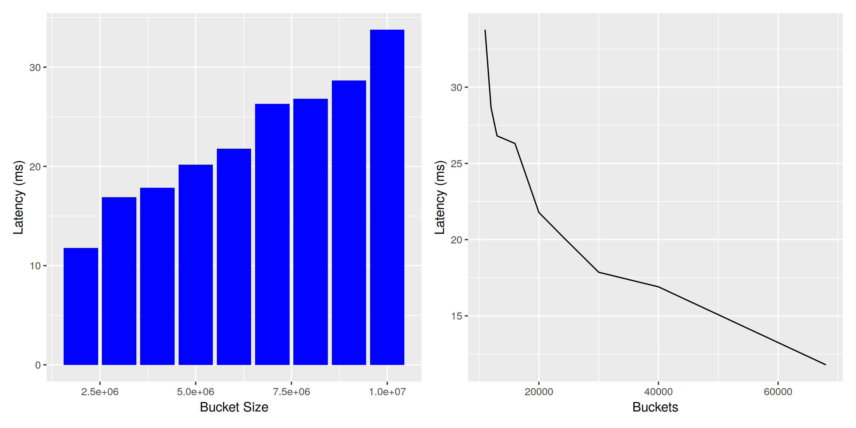Impact of changing buckets for query performance

The linear relationship between bucket size and query latency is visible in the plot, even though there seems to be some noise. The number of buckets is inversely proportional to the bucket size, so the associated plot is a shoddy approximation of $\frac{1}{x}$.

As a consequence, to improve query performance you can increase the number of buckets, at the expense of a reduced occupancy (see next subsection) and by making index maintainance more difficult (see next section). It is probably not useful to increase the number of buckets further when most partitions already have an individual bucket size of 2 or 3, as the disadvantages of having too many buckets start to outweigh the gains.

It’s also possible to increase the partition size while keeping the performance constant, if the number of buckets is increased alongside the values in each partition. This would allow replicating the query latency of 20ms even for larger index sizes, e.g. one trillion elements distributed over one million partitions.

Occupancy

To see the effect of the number of buckets on the occupancy of the index, we different indexes for a single partition with 100k elements, using buckets from [100 .. 100k) in steps of 500.

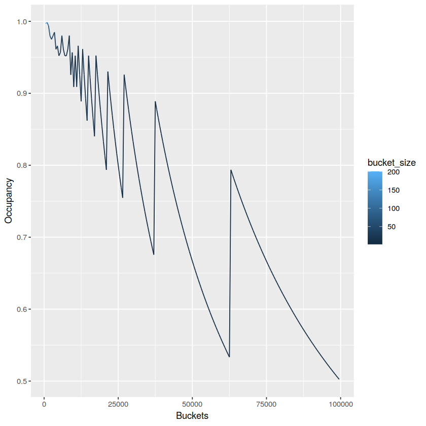Number of buckets vs occupancy

What’s happening here is that incrementing the number of buckets makes occupancy worse until a point where the partition data can fit in one less bucket, and occupancy jumps up. The occupancy is ideal near the peaks, but it’s not possible to optimize this for all partitions individually, as they all share the same number of buckets. The ideal bucket size thus depends on how big your partitions typically are, how much this size varies and how many partitions of each size you typically expect.

Concurrent Reads

It doesn’t seem promising to execute a single query on multiple CPU cores: while it’s in theory possible to walk over both bucket’s in parallel, or even split a bucket into smaller chunks, in reality the most expensive part is reading the data, in particular when data is persisted to typical cloud storage.

However, it should be easy to concurrently execute multiple queries. In this section, we’re looking into the effects of running 1, 2, 3, 4, 6 and 8 concurrent queries against a single index. Since the queries don’t get in the way of each other, we hope to see a linear scaling number of queries per second when increasing the number of readers.

We use an index with 1 million partitions, 100k entries each, and capture the query execution latency (i.e. a single thread running a single query), the query throughput (number of queries executed per second), and the read throughput (MB/s of data processed).

We expect the latency to stay constant (each thread does the same work, after all), and the throughput to scale linearly with the number of threads.

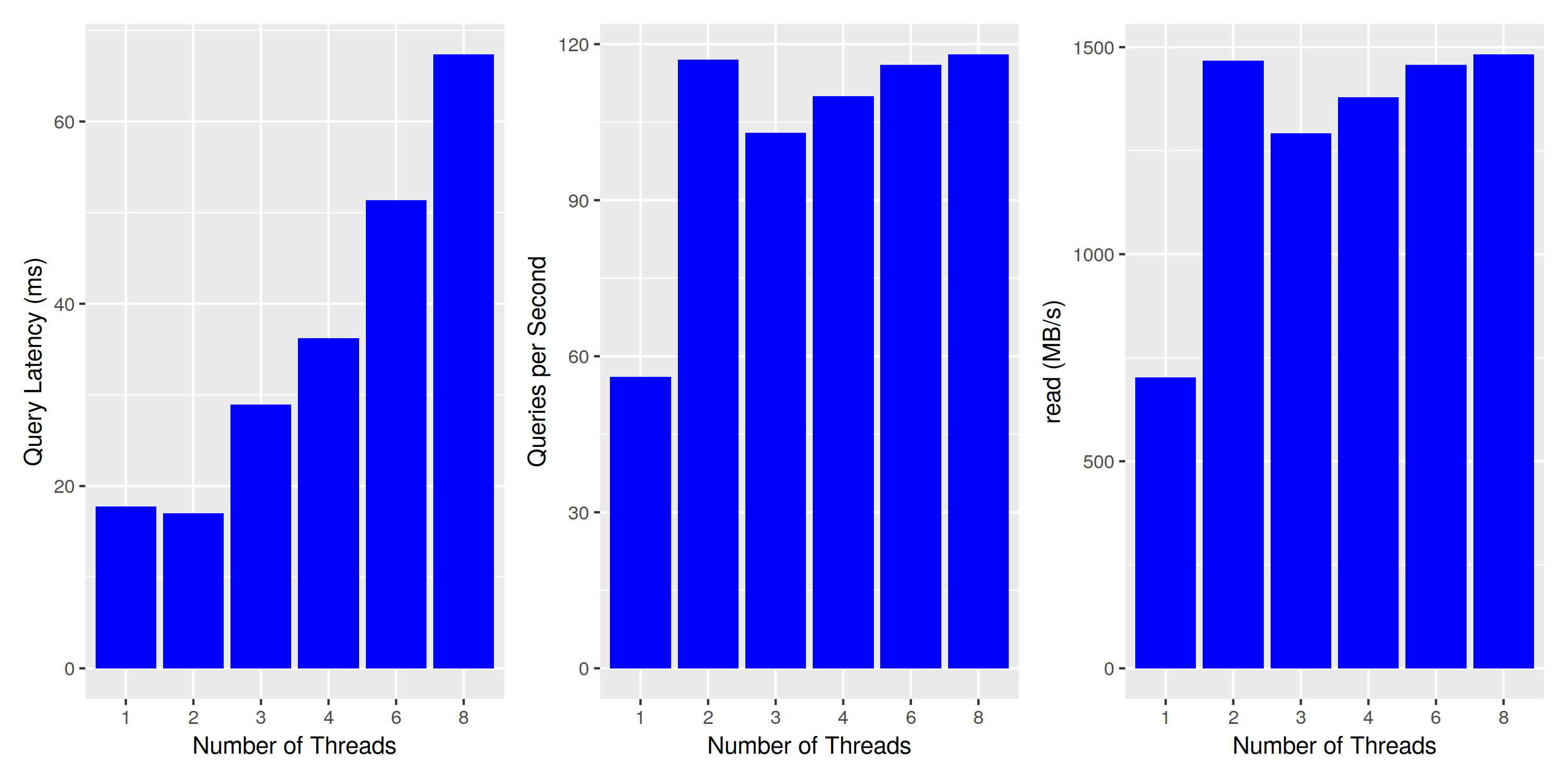Concurrent Query Execution: Where’s my scale?

This does not look good - query latency is not constant when executing multiple queries at the same time. To understand what’s going on, let’s look at the other two charts: queries per second and read bytes per second. Both are just different views into the same data, as each query reads exactly the same amount of data. However, this tells us that the number of queries is constant when running on two or more threads, and we might actually reach the limits of my laptop’s disk. While it’s specified to 3.5GB/s sequential reads, a quick test with hdparm yields 2.2GB/s - maybe this meager 1.5GB/s is all it can deliver when reading files of size 6MBs? To test our assumption, we re-run the same experiment with a reduced number of buckets, thereby increasing the bucket size:

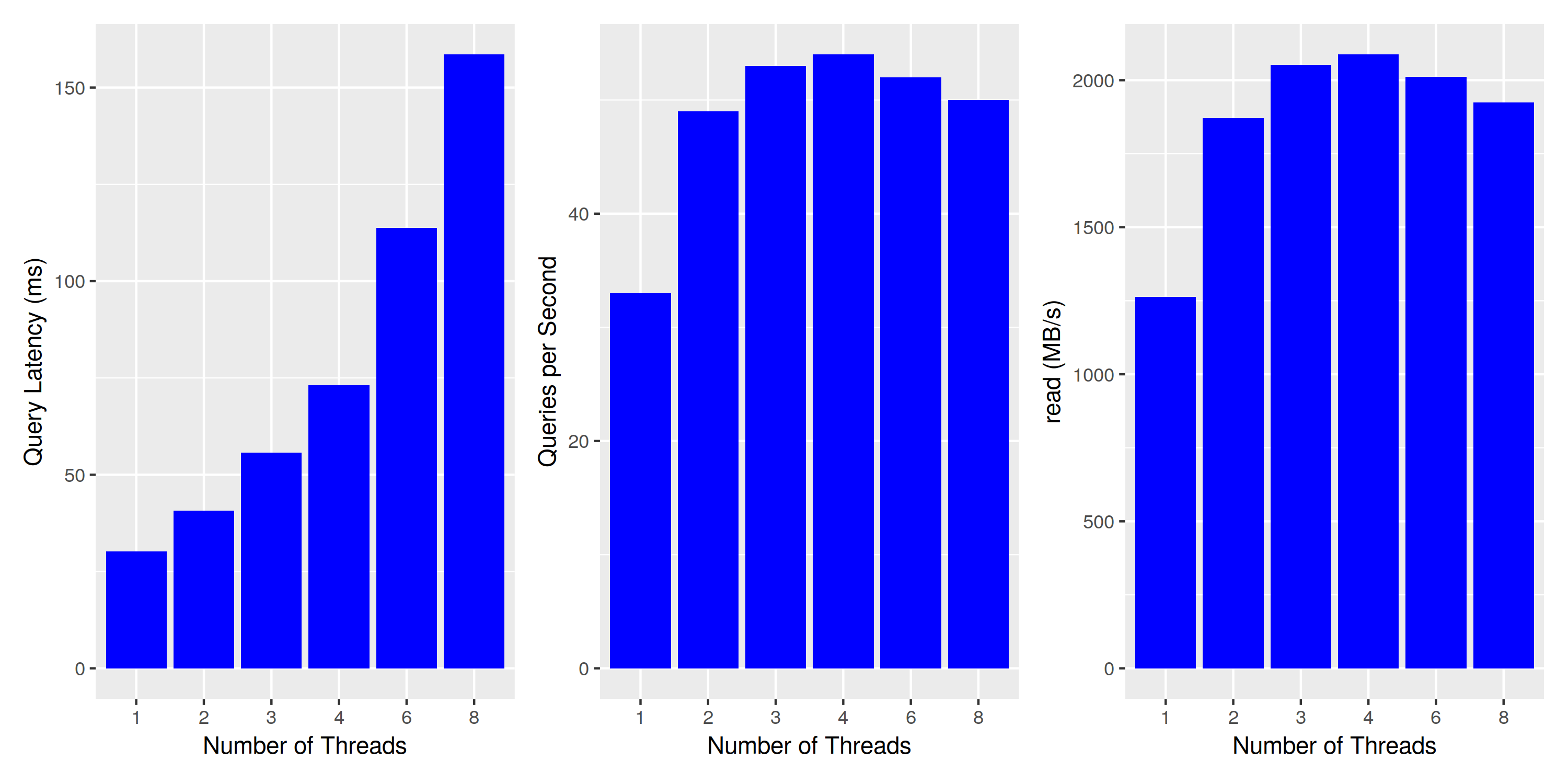Concurrent Query Execution: larger buckets increase throughput

Results are similar: single-threaded throughput is somewhat increased, as well as the overall disk throughput at about 2GB/s. To make sure we’re actually approaching the limits of the disk, we run one last experiment with a much smaller index size - reducing the number of partitions to 10k, thereby enabling it to serve all data from the file system cache:

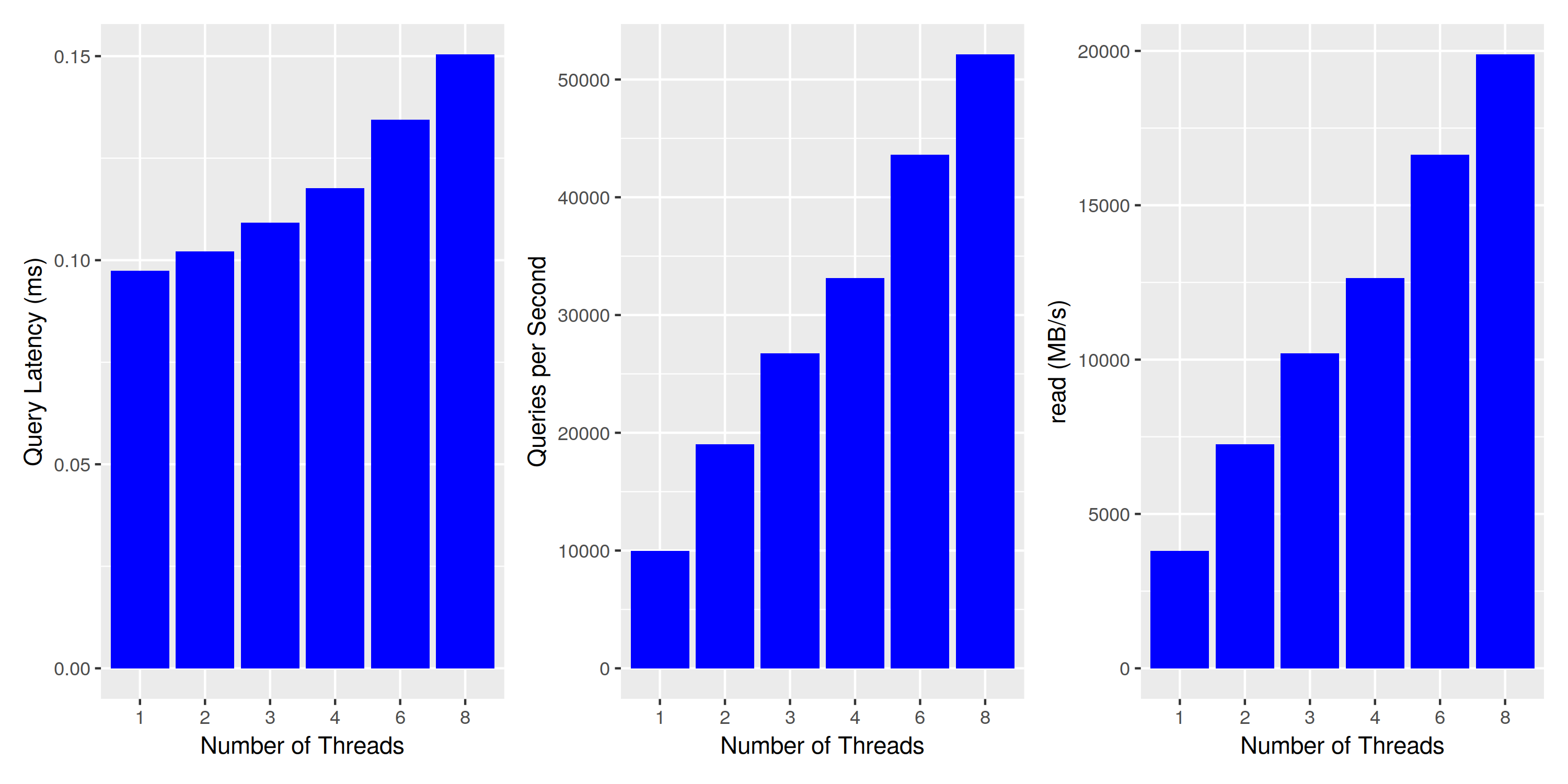Concurrent Query Execution: much higher throughput when data fits in the file cache

This looks much more reasonable. Throughput is scaling almost linearly with the number of threads, and the slowly increasing latency can be entirely explained by the decreased CPU clock in multi-core load situations (2.8 Ghz x 8 vs 4.3Ghz single-threaded).

False Positive Rate

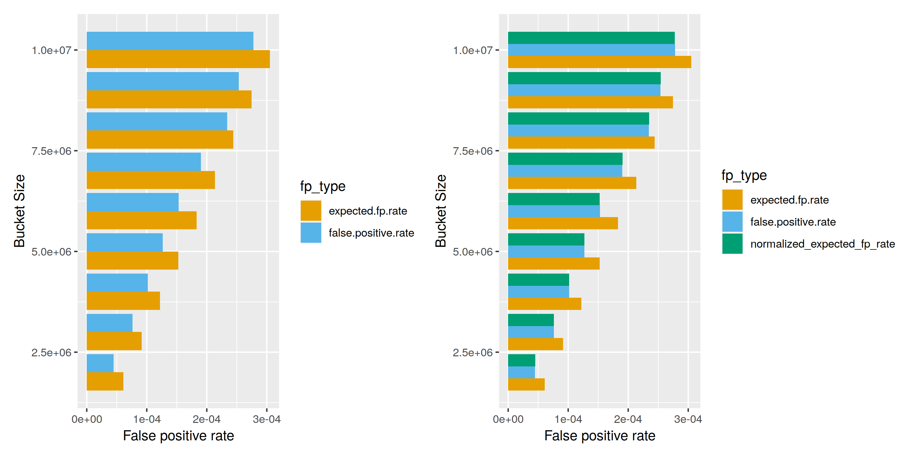
To make sure our index works as expected, we check that there are no false negatives (i.e. a query always produces the partition(s) owning the value) and also take a look at the false positive rate. As discussed previously, for a single cuckoo filter the expected false positive rate is $\text{fp} = \frac{2 b}{2^{fb}}$, where b is the. bucket size, and fb is the number of bits of the fingerprints.

False positive rate

I was initially surprised by the fact that the actual false positive rate was below the theoretical one, but later realized that the formula ignores vacant slots. On the right side, we normalized the expected false positive rate and multiply by the occupancy, which gives an almost perfect match between the experimentally tested and the theoretically expected false positive rate.

With an optimal bucket layout, we achieve a fp rate of 1 in 20000, which grows with a decreasing number of buckets. If we chose to represent fingerprints w/ 24 bits, we’d be looking at a very healthy false positive rate below one in a million, in exchange for an additional 50% of data in each bucket. However, the current implementation is kept simple and hard-codes the fingerprint width to 16 bits.

On Appending Data

Initially, we modelled the bucket data as one long, consecutive stream of bytes, writing data for successive buckets back to back. This layout makes it impossible to append additional files to the index structure, as there is simply no space between buckets to accommodate for the newly added fingerprints.

But this is not really necessary: buckets are always read independently, so it makes perfect sense to store the data for individual buckets in separate blobs or files. With that change in layout, appending data for a newly created partition requires appending the data for each bucket to its associated blob.

This is not a cheap operation; we’re appending a few fingerprints to thousands of different places. The behavior is somewhat expected: we optimized the data layout to serve queries with the minimum possible number of reads, and data is written predominantly by an orthogonal dimension (buckets vs partitions).

We don’t have a good solution for that problem: In our prototype, multiple writes are buffered to amortize writing bucket data. If the indexed data consists of immutable events, and the workload is read-heavy it may be worth maintaining an expensive index structure, which is a very similar trade-off to maintaining an index or a materialized view in any database system.

Buffering data also introduces all the pitfalls and complexities we all loathe love from distributed systems: when buffering writes in memory, we probably need some sort of write-ahead log of new index data, likely in the form of appending the original cuckoo filter data as a per-partition blob, and a way to restore that WAL on crash recovery.

Prior Art

After explaining my idea to a coworker, he pointed me to COBS - compact bit-sliced signature index. The authors are using a very similar approach, but there’s a few noteworthy differences.

COBS uses Bloom filters in the context of finding DNA sequences in a large body of samples. A query typically involves a variable-sized subsequence of DNA, and indexing happens on k-mer level. Since the actual search involves far longer sequences, a search query is translated into a conjunction of many k-mers. This implies that the false positive rate of the index itself doesn’t have to be very low, as false positives get weeded out via the conjunction of many search terms. In such a scenario, you can get away with just a single hash function. This wouldn’t be feasible in our scenario: we assume that a query is searching for a single value. Using Bloom filters for our partition index would lead to either high false positive rates or a large number of hash functions: to achieve a false-positive rate of 1 in 20000, a Bloom filter needs k = 14 hash functions, requiring 14 I/O operations to evaluate a query.

To save space and incorporate documents (files or partition in our terminology) of variable size, Bloom filters are not aligned to one specific length. Instead, Bloom filters are grouped together with other, similarly-sized documents, resulting in multiple aligned “blocks” of different sizes. This reduces the size of the index, but further increases the number of I/O operation, because you’d have to perform k I/O operations for each block of filters. We avoid doing this by enabling a variable bucket size per cuckoo filter, so there’s only one big block of buckets, but false positive rates and occupancy vary for partitions depending on their size.

The paper also introduces “ClaBS”, which does away with the “compact” representation via multiple aligned blocks, described in the previous paragraph, and is closer to the partition index described in this blog post. In the benchmark section, they compare ClaBS and COBS with other approaches, but all measurements are done in-memory, so the theoretical I/O advantage of ClaBS over COBS does not materialize, and the latter shows supreme performance behavior.

Writing COBS is even harder than writing our partition index: appending a single partition requires adding a single bit to all slices, which is even worse than appending several fingerprints of 16 bits each to all buckets.

Conclusion

If you made it that far - thank you very much. This was my first “personal” blog post, and it is a lot longer than initially anticipated. It also took a lot longer to write, mostly because when actually writing down your ideas you get a lot of back-and-forth with yourself, and it’s pretty hard to stop.

As for the approach itself, I’m interested in feedback - maybe something very similar is already built into some query engines? If not, I’d really love to to see it materialize as part of a proper query engine. In particular, I’d love to see the performance that can be achieved in conjunction with Parquet files: Just imagine what levels of performance are possible when combined with the techniques described in the Influx Data blog post “Querying Parquet with Millisecond Latency”.

Future work

At the moment, all we have is a basic Rust library to verify the initial idea. There are too many open ends to list them all, but here’s some starting points:

• robust, fault-tolerant write path
• solve consistency when interacting with another system (e.g., a proper query engine)
• optimize performance: SIMD, async, … lots of things that have been neglected so far
• some sort of REST API to make this a stand-alone component in a larger system
• look into more advanced approximate membership query algorithms, e.g. taffy filters and vacuum filters